Sulfur dioxide pollution has fallen by 95 percent in the US

Super fact 44 : Sulfur dioxide pollution has fallen by approximately 95 percent in the US since the 1970s. This significant reduction is primarily due to regulations like the Clean Air Act. Global sulfur dioxide pollution has also fallen but not as much.

Sulfur dioxide is a colorless gas with the formula SO2. It has a pungent smell, which you notice after using matches. It is released naturally by volcanic activity and is produced as a by-product of burning sulfur-bearing fossil fuels and from metals refining. Sulfur dioxide is somewhat toxic to humans and by reacting with water it creates acid rain, which is a serious environmental problem.

The good news is that the Clean Air Act has driven technological advancements and the adoption of cleaner practices in industries that produce sulfur dioxide emissions. This has resulted in a drop of sulfur dioxide pollution in the US by 95% according to EPA and Statista and 94% according to Our World In Data. Statista is a pay site, so I am not going to link to it. Below is a graph from Our World In Data showing the reduction in sulfur dioxide pollution in the US.

The graph shows a steep increase towards the end of the 19th century with a peak in 1973, followed by a steep decline | Sulfur dioxide pollution has fallen by 95 percent in the US
US sulfur dioxide pollution since 1800. Data Source: Hoesly et al (2024) – Community Emissions Data System (CEDS). This graph is taken this page in Our World In Data.<<Link-5>> US Emissions peaked in 1973.

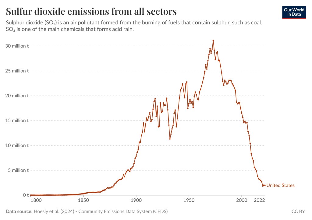
I should mention that by clicking this link you can visit the graph above Our World in Data and select different countries and regions and play around with the settings.

Sulfur Dioxide Emissions Worldwide

The worldwide emissions peaked in 1979 and fell sharply after that even though the progress (reduction in sulfur dioxide emissions) has not been as spectacular as in the US. Worldwide reductions are around 48%. Again, by visiting the Our World In Data page you can play around with the graph and the settings and view different countries and regions. This is an additional source visualizing the data.

The graph shows a steep increase in sulfur dioxide emissions around 1950 with a peak in 1979, followed by a steep decline, but not as dramatic as for the US
Sulfur dioxide pollution worldwide since 1800. Data Source: Hoesly et al (2024) – Community Emissions Data System (CEDS). This graph is taken this page in Our World In Data. Worldwide Emissions peaked in 1979.
This graph shows the sulfur dioxide emissions for the world as well as for China and India. China follows the world wide emissions but on a smaller scale whilst India has steady increase in emissions that stabilized/peaked in 2023 | Sulfur dioxide pollution has fallen by 95 percent in the US
Sulfur dioxide pollution worldwide since 1800 with three major polluters included. The United States is in red, China in green and India in blue. The graph for India is the one corresponding to the least overall pollution but it has no reduction. Data Source: Hoesly et al (2024) – Community Emissions Data System (CEDS). This graph is taken this page in Our World In Data.

Good News with Respect to Pollution

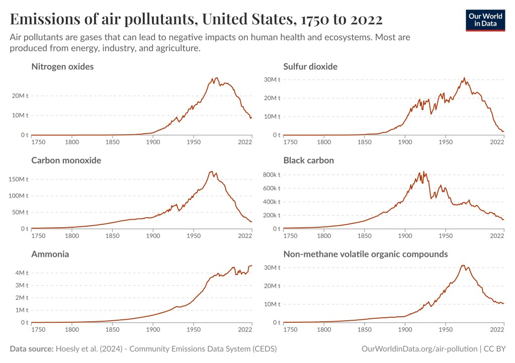
Sulfur dioxide emissions have gone down worldwide, which is good news. However, sulfur dioxide is not the only pollutant that we have succeeded in reducing. The graph below demonstrates that the US has also made great progress in reducing Nitrogen Oxides pollution, Carbon Monoxide, Black Carbon, and Non-methane volatile organic compounds. We have not been as successful with reducing Ammonia pollution.

However, according to Google AI sulfur dioxide, followed by Nitrogen Oxides pollution, Carbon Monoxide, and Black Carbon are the most serious pollutants. The graph below is taken from this page in Our World in Data.

The graphs for nitrogen oxide emissions, sulfur dioxide emissions , carbon monoxide and non-methane organic compounds pollution peak around 1970’s and then show a sharp downturn. The graph for black carbon peak around 1920 and then show a sharp downturn whereas the graph for ammonia does not peak. All graphs are in red.
US nitrogen oxide emissions, sulfur dioxide emissions, carbon monoxides, black carbon, ammonia and non-methane organic compounds pollution since 1750. Data Source: Hoesly et al (2024) – Community Emissions Data System (CEDS). This graph is taken from this page in Our World In Data.

The graphs for the world do not look as impressive. However, even in this case it looks like some progress has been made. Four graphs have peaked and are turning downwards, and one graph has flattened but unfortunately the graph for ammonia pollution is still heading upwards.

It should be noted that these pollutants are more or less local in the sense that they affect the polluting country and/or surrounding countries the most, whilst the climate change / global warming effect from carbon dioxide and other long lasting greenhouse gases tend to affect the entire planet.

The graphs for nitrogen oxide emissions, sulfur dioxide emissions , carbon monoxide peak around 1970’s and then show a small downturn. The graph for black carbon peak around 2020 and then shows a small downturn. The graph for non-methane organic compounds pollution flattened around 2020 whereas the graph for ammonia keeps growing. All graphs are in blue | Sulfur dioxide pollution has fallen by 95 percent in the US
Worldwide nitrogen oxides emissions, sulfur dioxide emissions, carbon monoxide emissions, black carbon, ammonia and non-methane organic compounds pollution since 1750. Data Source: Hoesly et al (2024) – Community Emissions Data System (CEDS). This graph is taken from this page in Our World In Data.

Aside from the success in reducing these pollutants there is more good news.


To see the other Super Facts click here

The US is the largest cumulative emitter of carbon

Super fact 43 : The United States has emitted more CO2 than any other country to date, around 400 billion tons since 1751. It is responsible for 25% of historical emissions. Click here.

But what about China? That is 12.7%, or around half. This is surprising information to many Americans, yet it is true, and therefore a super fact. In the US it is very common to blame China for our carbon emissions. In China they blame the US. In Europe they blame the US and China. Who is right? It turns out that the blame game is complicated and futile.

Carbon Emissions Around the World

Who should we blame the most for our carbon emissions?

In other words, if you want to blame another country for the carbon emissions, take your pick, well your cherry pick. Why should we do something about our carbon emissions when X is worse? Those who want no action on the global warming / climate change problem love the blame game. Like denial or despair, which are both irrational positions, the blame game hinders action. The blame game can also get very complicated and contentious.

The nine graphs are complex but show that among the nine countries/regions the United States currently has the highest emissions, followed by Canada, and the China, then South Africa, then the European Union, then comes the United Kingdom, and the World, and finally India and Kenya | The US is the largest cumulative emitter of carbon
The graph shows the fossil fuel emissions (in carbon dioxide equivalents) per capita from 1750 to 2023 for the World, the United States, Canada, China, European Union, India, South Africa, United Kingdom, and Kenya. Notice that the United Kingdom dominated the emissions in the 1700’s and 1800’s. Data source: Global Carbon Budget (2024); Population based on various sources (2024). The graph is from Our World in Data .

Note regarding the graph above: By clicking here you can find this graph and then select to display any set of countries or regions. Have fun experimenting.

Note regarding Fossil emissions: Fossil emissions measure the quantity of carbon emissions (CO2) emitted from the burning of fossil fuels, and directly from industrial processes such as cement and steel production. Fossil CO2 includes emissions from coal, oil, gas, flaring, cement, steel, and other industrial processes. Fossil emissions do not include land use change, deforestation, soils, or vegetation.

Overview of Cumulative Carbon Emissions

As you can see in the graph below the cumulative carbon emissions from 1751 to 2017 are 25% for the United States, 22% for the EU (28 countries), 12.7% for China, 6% for Russia, 4% for Japan, and 3% for India. If you count the entire continent of Europe, you get 33% for Europe.

The graph shows differently colored rectangles with the area of the rectangle corresponding to the cumulative carbon emissions. Each rectangle corresponds to a country or a region.
Figures for the 28 countries in the European Union have been grouped as the EU-28 since international targets and negotiations are typically set as a collaborative target between EU countries. Values may not sum up to 100% due to rounding. Data Source: Calculated by Our World in Data from the Global Carbon Project (GCP) and Carbon Dioxide Analysis Center (CDIAC). This is a visualization from Our World in Data, where you can find data and research on how the world is changing.
To see the other Super Facts click here

Developed nations have successfully reduced carbon emissions

Super fact 42 : The developed nations (rich countries) have reduced their carbon emissions since the 1990’s despite continued GDP growth, even if we take offshore production into account. In addition, many developing countries have succeeded in reducing their emissions as well. Other fast-growing developing countries have flattened or at least slowed their increase in carbon emissions. Many countries have decoupled economic growth from CO2 emissions. In other words, we do not need to increase carbon emissions or burn more fossil fuels to grow the economy.

This is good news as well as a surprise to many people who falsely believe that to grow the economy (grow GDP) you need to burn more fossil fuels and an increase in carbon emissions is inevitable if you want to grow the economy. The data shows otherwise. This is important news that is difficult to believe in for many people. It is a super fact.

Carbon Emissions and GDP

In the past carbon emissions were strongly correlated with national wealth. The wealthier a nation was the higher its carbon emissions were and as the economy grew so did the carbon emissions. This has not been true since the 1990’s. The developed nations of the world have continued growing their GDP whilst reducing their carbon emissions.

You may think that the reason is that we shipped much of our manufacturing overseas and that if you consider the consumers in the importing country responsible for the overseas emissions this decoupling of GDP and emissions would disappear. But you would be wrong. Even if you make the consumers in the importing country responsible for the emissions during production in the exporting country the emissions have gone down. One example taken from this article in Our World in Data is the United Kingdom.

In the graph below for the UK the GDP (adjusted for inflation) grew by 53.26% between 1990 and 2023 and the emissions were reduced by 57.66%. If make UK consumers 100% responsible for the emissions in China and India, etc., caused by the production of goods imported to the UK the reduction until 2022 was 38.59%. That is not as much but it is still impressive and demonstrates the decoupling between GDP growth and carbon emissions.

The graph shows three plotted graphs, a dark blue one showing GDP per capita, a light blue one showing UK carbon emissions per capita and a red one showing trade adjusted carbon emissions per capita. The GDP graph is increasing by more than 50% over 33 years and the CO2 emissions per capita graph is decreasing by almost 60% and the trade adjusted carbon emissions decline by almost 40% | Developed nations have successfully reduced carbon emissions
Data source: Data compiled from multiple sources by World Bank (2025); Global Carbon Budget (2024); Population based on various sources (2024). Note: GDP per capita is expressed in international dollars at 2021 prices. Graph taken from Our World in Data.

The text in the graph above is difficult to read so I’ve copied it below in larger text:

  • Consumption-based emissions: Consumption-based emissions are national or regional emissions that have been adjusted for trade. They are calculated as domestic (or ‘production-based’ emissions) emissions minus the emissions generated in the production of goods and services that are exported to other countries or regions, plus emissions from the production of goods and services that are imported. Consumption-based emissions = Production-based – Exported + Imported emissions.
  • Fossil emissions: Fossil emissions measure the quantity of carbon dioxide (CO2) emitted from the burning of fossil fuels, and directly from industrial processes such as cement and steel production. Fossil CO2 includes emissions from coal, oil, gas, flaring, cement, steel, and other industrial processes. Fossil emissions do not include land use change, deforestation, soils, or vegetation.
  • International dollars: International dollars are a hypothetical currency that is used to make meaningful comparisons of monetary indicators of living standards. Figures expressed in constant international dollars are adjusted for inflation within countries over time, and for differences in the cost of living between countries. The goal of such adjustments is to provide a unit whose purchasing power is held fixed over time and across countries, such that one international dollar can buy the same quantity and quality of goods and service no matter where or when it is spent. Read more in our article: What are Purchasing Power Parity adjustments and why do we need them?

Below is the same type of graphs for the United Kingdom as well as France, Germany, Sweden, United States and Finland. The numbers for these countries are as follows:

  • United Kingdom: GDP growth 53.26%, CO2 emissions reduction 57.66%, trade adjusted CO2 emissions reduction 38.59%.
  • France: GDP growth 39.74%, CO2 emissions reduction 40.64%, trade adjusted CO2 emissions reduction 28.82%.
  • Germany: GDP growth 49.04%, CO2 emissions reduction 46.72%, trade adjusted CO2 emissions reduction 33.95%.
  • Sweden: GDP growth 56.00%, CO2 emissions reduction 48.45%, trade adjusted CO2 emissions reduction 34.75%.
  • United States: GDP growth 68.05%, CO2 emissions reduction 29.25%, trade adjusted CO2 emissions reduction 17.04%.
  • Finland: GDP growth 45.69%, CO2 emissions reduction 50.54%, trade adjusted CO2 emissions reduction 42.79%.

Note these are emissions reduction numbers per capita (growth for GDP) not carbon emissions per capita. For example, the United States has three to four times larger carbon emissions per capita as, for example, Sweden or France.

All these graphs show the same trends as the UK graph.
Data source: Data compiled from multiple sources by World Bank (2025); Global Carbon Budget (2024); Population based on various sources (2024). Note: GDP per capita is expressed in international dollars at 2021 prices. Graph taken from Our World in Data.

Many Countries Have Reduced Their Carbon Emissions

However, the story does not end with these six countries or even with the developed world. The 30 graphs below all demonstrate significant reductions in carbon emissions as GDP is growing, demonstrating a decoupling between GDP growth and carbon emissions. Note that Azerbaijan’s GDP grew by 93% as its carbon emissions was reduced by 7% (all carbon emissions below are adjusted for trade).

This is 30 small graphs featuring a blue and red line. The blue line shows GDP growth since 1990 and the red line carbon emissions since 1990. All blue lines point up and all red lines point down | Developed nations have successfully reduced carbon emissions
Data sources: Global Carbon Project & World Bank. There are more countries that achieved the same, but only those countries for which data is available and for which each exceeded 5% are shown. The graphs are from Our World in Data <<Link-1>>. All carbon emissions in the graphs above are adjusted for trade.

The World’s Carbon Emissions Per Capita Has Flattened

World GDP per capita has increased by 83.54% since 1990 while carbon emissions per capita have grown by 9.48%. That may not be as impressive but note two things. That is still a decoupling between economic growth and if you look in the graph, you’ll see that carbon emissions were higher in 2008 to 2019. The curve has flattened and gone down a bit. Global Warming caused by our burning of fossil fuels may be the greatest environmental challenge in recorded history, but we are slowly and steadily turning things around. We are not doing it fast enough to avoid major damage to our eco systems and perhaps civilization, but we are still turning things around. If you have any doubts about global warming / climate change or that we are causing it click here for a summary of the evidence.

The graph shows two graphs. The dark blue one shows GDP growth per capita and the light blue the carbon emissions per capita.
Data source: Data compiled from multiple sources by World Bank (2025); Global Carbon Budget (2024); Population based on various sources (2024). The graph is taken from Our World in Data <<Link-1>>.

China’s Carbon Emissions

One reason the world’s carbon emissions per capita have not been reduced much despite the fact that so many countries have reduced their emissions is that the world’s largest emitter China, has grown their carbon emissions steadily since 1990. Between 1990 and 2023 China’s GDP per capita (and adjusted for inflation) grew by 1,245.28% and their emissions grew by 288.43% per capita. Remember that China has 1.4 billion people so that is a big carbon blast for the world.

However, before you blame China too much remember that China’s carbon emissions per capita is less than that of the United States and that of many other developed countries, and the country with the largest cumulative carbon emissions is the United States. China’s economic growth has been immense, and its immense population of 1.4 billion people explains its huge impact on the world’s carbon emissions.

Fortunately, it now appears that China’s emissions have finally peaked.

To see the other Super Facts click here

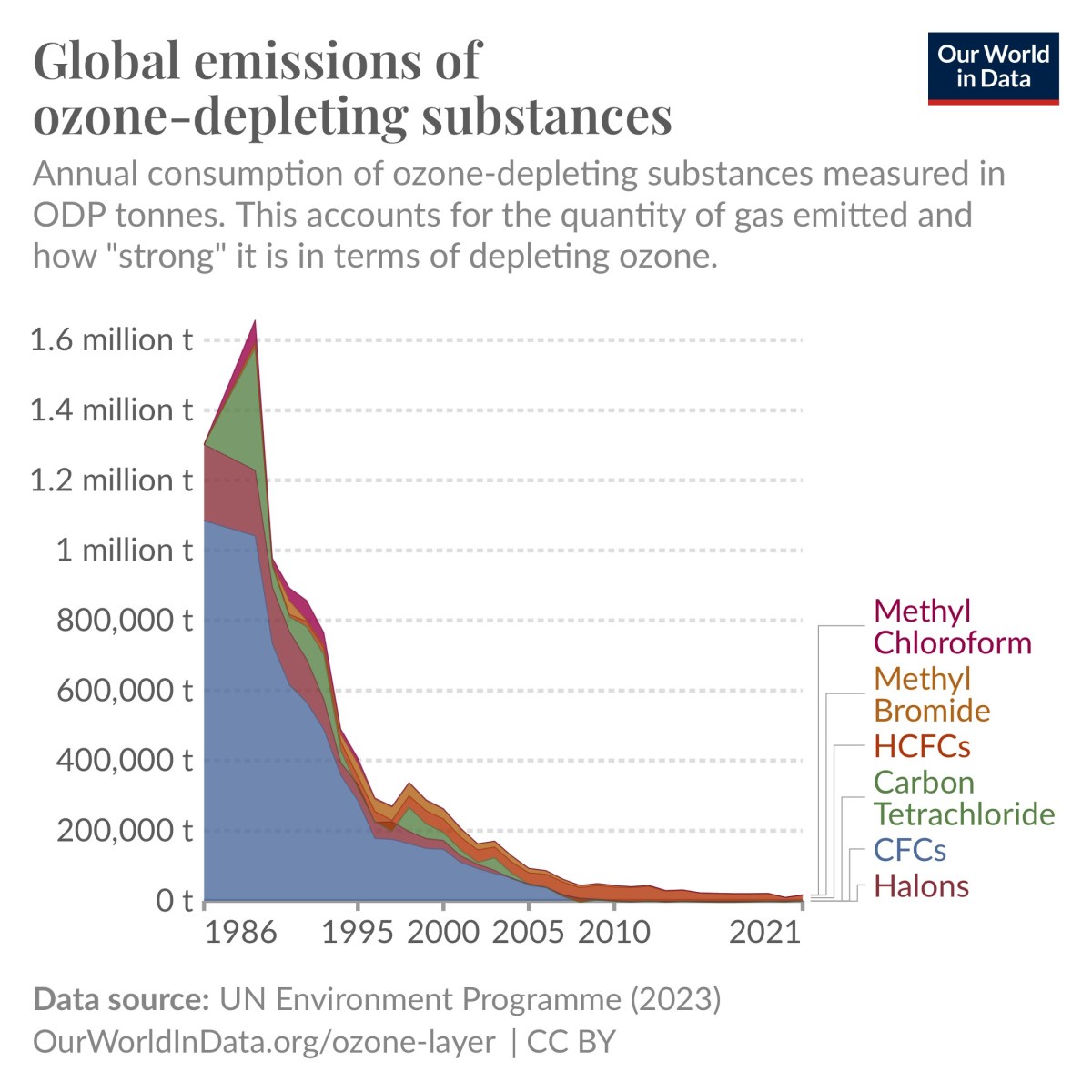
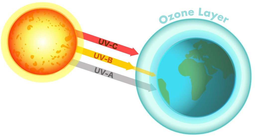
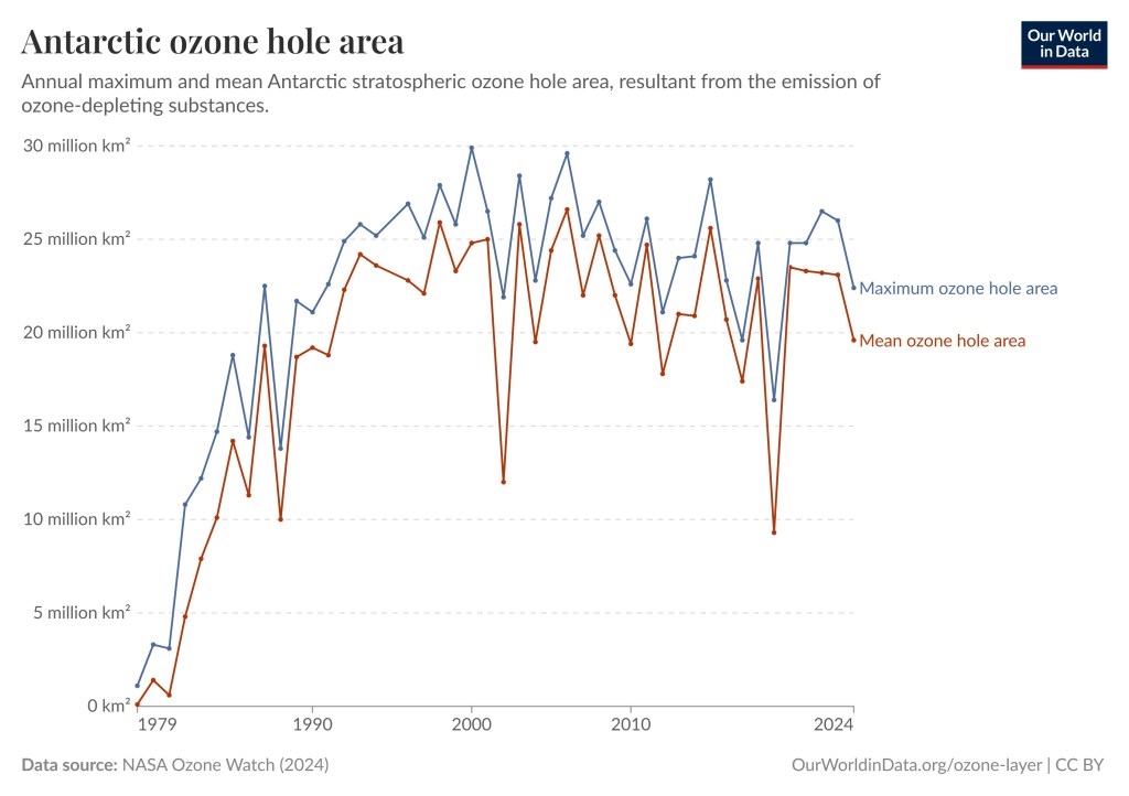
Emissions of ozone-depleting gases have fallen by 99 Percent

Super fact 41 : Largely thanks to the Montreal Protocol in 1987 the emissions of ozone-depleting gases have fallen by more than 99%, 99.7% to be exact, according to Our World in Data. This has resulted in halting the expansion of the ozone holes and the reduction in emissions of  ozone-depleting gases is saving millions of lives every year.

This is my good news for Earth Day, and it is a super fact. It is a super fact because a lot of people believe that the issue with ozone depleting gases and Montreal protocol is bunk. They take the fact that we are not talking about it much nowadays as evidence that there was nothing to it in the first place. However, they are wrong. We typically don’t talk much about environmental problems that have been addressed successfully. The Antarctic ozone hole that we used to worry about is still there, but its worrisome expansion has been halted.

The Reduction of Ozone-Depleting Gases

The ozone layer, located in the stratosphere, protects Earth from harmful UV radiation. Ozone (O3) is naturally created and destroyed in a balance, but ozone-depleting substances damage the ozone layer by releasing chlorine atoms that catalyze the destruction of ozone molecules.

This problem was discovered by Mario Molina and F. Sherwood Rowland in 1974. They were awarded the 1995 Nobel Prize in Chemistry, along with Paul Crutzen, for their work in atmospheric chemistry. Examples of ozone depleting gases are chlorofluorocarbons (CFCs), hydrochlorofluorocarbons (HCFCs), halons, methyl chloroform ,methyl bromide, carbon tetrachloride, hydrobromofluorocarbons, and chlorobromomethane.

The picture shows the sun radiating UV radiation to earth, which is protected by a blanket of ozone | By 2018 the emissions of ozone-depleting gases had fallen by 99.7 percent
Ozone layer depletion diagram. Earth’s sunscreen, shielding us from the sun’s harmful ultraviolet rays. UV A, B, C. UVA, UVB, UVC.

Ozone depletion causes a breakdown of the ozone layer around the world, including the famous Arctic and Antarctic ozone holes. This allows more UV radiation to reach Earth surface, increasing the exposure to harmful ultraviolet (UV) radiation, which can cause skin cancer, cataracts, and immune system damage.

It also harms plants and marine life, as well as climate. It should be noted that this is a different problem from climate change or if you call it global warming, even though ozone depletion to some degree influence climate change. You can read about climate change related super facts here, here and here.

The Reduction of Ozone-Depleting Gases

The good news is that we have been very successful in reducing ozone depleting gases. The Montreal protocol, a landmark international agreement signed in 1987 to protect the Earth’s ozone layer by phasing out ozone depleting gases, has been very successful.

As you can see in the diagram below from Our World in Data. We have had at least a 99% reduction in ozone depleting gases according to the NASA, the World Economic Forum and the UN Environment Program. More specifically, the reduction is 99.7% by 2018 according to Our World in Data.

Gases visualized in the diagram are CFCs, Halons, HCFCs, Carbon Tetrachloride, Methyl Bromide, Methyl Chloroform. The diagram shows a peak around the end of 1980’s | By 2018 the emissions of ozone-depleting gases had fallen by 99.7 percent
The phase out of six ozone depleting gases. Data source UN Environment Program (2023).

443 million Cases of Skin Cancer Prevented

The NIH estimate that the Montreal Protocol has prevented 443 million cases of skin cancer, 2.3 million skin cancer deaths, and 63 million cases of cataracts in the United States alone. Globally, it is estimated that the Protocol has saved an estimated 2 million people from dying from skin cancer each year.

Yes, you can read that again :

Worldwide the Montreal Protocol has saved an estimated 2 million people from dying from skin cancer each year.

To read more about the Montreal Protocol and the ultimate repair job click here.

The Antarctic Ozone Hole

What about the Arctic and Antarctic ozone holes? Well, they are not gone but they are retreating. When there is an environmental problem, it does not entirely disappear right away even if you remove the root cause. The same is true for global warming. If we succeeded to stop all carbon emissions tomorrow it would take decades for average temperatures to stop rising and hundreds of years for them to come down to “normal”. But remember it would have been much worse without the Montreal Protocol.

There are two graphs. The graph representing the annual mean Antarctic ozone hole is blue.  The graph representing the annual maximum Antarctic ozone hole is red. Both graphs are rising initially but after the year 2000 the graphs flatten and even go down a bit.
The graph is from Our World in Data and data comes from NASA Ozone watch 2024.
To see the other Super Facts click here

The Surprising Butterfly Effect

Super fact 40 : In chaotic systems the so-called butterfly effect means that a small change in initial conditions, such as a butterfly flapping its wing in Brazil, can lead to large, unpredictable changes in a system’s future, such as the appearance of a tornado in North Texas. However, that does not mean that the butterfly directly caused the tornado. It should also be noted that chaotic systems can contain predictable patterns and external forcings can certainly make aspects of a chaotic system behave in a predictable manner.

The first part of Super Fact 40 describes a well-established phenomenon that is often surprising to people who have not heard about it before. The second part (following the word “However”) address a few common misconceptions about the butterfly effect. The butterfly effect is a surprising and widely misunderstood phenomenon and therefore I consider the information in bold above to be a super fact.

The Surprising Butterfly Effect
Photo by Cindy Gustafson on Pexels.com

The Butterfly Effect and Unpredictability

The butterfly effect is the sensitive dependence on initial conditions in which a small change in one aspect of the system can result in large differences later. A butterfly flapping its wing in Brazil, leading to the appearance of a tornado in North Texas, is one example. The butterfly effect is an aspect of chaos theory.

However, it is important to understand that the butterfly is not directly causing the tornado. It is the wing flaps of trillions of butterflies, the wing flaps of 50 billion birds, the barks of 900 million dogs, all the waterdrops in the world, and all the bushes and trees, etc., which together provide the initial conditions for the world’s weather system.

Remove one butterfly, anyone of them, or the bark of a dog, and you may or may not have a tornado in north Texas on a certain date. It isn’t the butterfly causing the tornado. Any tiny change in the initial conditions will eventually lead to a large difference in the system later. This is how the Butterfly Effect provides unpredictability.

A large well-formed tornado over the plains.
Did a butterfly do this? Stock Photo ID: 2369175167 by g images.com.

The Butterfly Effect and Predictability

Because of the butterfly effect you may not be able to predict whether it is going to rain at 1:00PM next Thursday, but you can still safely predict that Dallas, Texas, will on average be cooler in January than in July. That’s largely because the sun will heat Dallas, Texas more in July than in January. We know that if you add carbon dioxide, or other heat trapping gases, to the atmosphere it will on average get warmer. External forcings make aspects of chaotic systems predictable. You sometime hear the argument that “climate is chaotic and cannot be predicted”. This is a myth that is debunked here.

In addition, chaotic systems can feature predictable patterns, even though chaotic systems are considered unpredictable. Chaos theory demonstrates that within the apparent randomness of chaotic systems, there are underlying statistical patterns, self-similarity, fractals, and interconnection.

I once created a robot control system for which the robot was shaking a little bit. The tool tip was moving in a little circle and did not get to where it was supposed to be. The reason was that the presence of static friction made the control system I was using a chaotic system.

However, the robot didn’t randomly go all over the place. It was moving quickly in a small circle. It was chaotic, and its exact motion was unpredictable, but there was an underlying statistical pattern. Another example is, fractals, which are geometric patterns that emerge from chaotic processes described by chaos theory. Fractals feature self-similar patterns repeating at different scales. They can visually represent the complex behavior of these systems. See an example below.

A 450 layer fractal | The Surprising Butterfly Effect
This is a file from the Wikimedia Commons Wikipedia. Simpsons contributor at English Wikipedia, Public domain, via Wikimedia Commons.

Edward Norton Lorenz

In 1961, Edward Norton Lorenz was using a computer to simulate weather patterns by modeling 12 variables (heat, wind, etc.). After finishing one simulation he wanted to see it again but to save time he started it in the middle using the saved variables at the point. To his surprise his simulation ended up with completely different weather. He realized that the computer the saved data had tiny errors from the computer rounding off the numbers. For example, 3.145787 instead of 3.1457872. That small difference was enough to eventually result in completely different weather.

Lorenz was not the first person to realize that, so called, non-linear systems can be extremely  sensitive initial data. This realization goes all the way back to the mathematician Henri Poincaré in the 19th century. However, he was the founder of modern chaos theory and coined the term the Butterfly Effect.

To see the other Super Facts click here

What do you think about the Fractal above?